Peigen Zhou 15 Oct 2017

R Markdown / stan

Stan is one of my faviorate programming language, there are tones of people using stan as daily research or analysis purpose, Facebook’s new pacakge PROPHET.

Install R package rstan

Rstan is the R interface to stan, which using for statistical modeling, data analysis, and prediction in the social, biological, and physical sciences, engineering, and business.

This tutorial will introduce how to install R stan into our computer and how to use R stan in real problem.

install.packages("rstan")
library(rstan)

Genetic Linkage Model

Suppose that 197 animals (Y) are distributed into four categories as follows: \[Y = (y_1, y_2, y_3, y_4) = (125, 18, 20, 34)\] with cell probabilities \[(\frac{1}{2} + \frac{\theta}{4}, \frac{1}{4}(1-\theta), \frac{1}{4}(1-\theta), \frac{\theta}{4})\]

The EM algorithm will use augment method to make the likelihood function easy to me maximized. So how to put the question into stan?

Model file or code: Stan has 7 main blocks:

functions Define your own function, likelihood, sampling distribution
data Using for input data
transformed data
parameters Parameters need to estimate
transformed parameters
model As its name
generated quantities Some quantities you are interested

linkage_code <- '
data {
  int<lower=0> y[4];
}

parameters {
  real<lower=0, upper=1> theta;
}

transformed parameters {
  vector[4] ytheta;
  ytheta[1] = 0.5+theta/4;
  ytheta[2] = 0.25-theta/4;
  ytheta[3] = 0.25-theta/4;
  ytheta[4] = theta/4;
}

model {
  y ~ multinomial(ytheta);
}
'

y <- c(125, 18, 20, 34)
dat <- list()
dat$y <- y

First we compile our model to a S4 stanmodel object.

model_obj <- stan_model(model_code = linkage_code, model_name = "GeneticLinkage")

Sampling

fit <- sampling(model_obj, data = dat, iter = 1000, chains = 4)

you can also save your model_code into a file maybe call “genetic.stan”, then use argument file = "gentic.stan".

iter means length of chains, chains means how many chains you want to use.

You can use a list to store all the data, then put them into your stan model.

Some inference

First you may need to check is whether the Markov chains are converged.

print(fit)

## Inference for Stan model: GeneticLinkage.
## 4 chains, each with iter=1000; warmup=500; thin=1; 
## post-warmup draws per chain=500, total post-warmup draws=2000.
## 
##              mean se_mean   sd    2.5%     25%     50%     75%   97.5%
## theta        0.62    0.00 0.05    0.52    0.59    0.62    0.66    0.72
## ytheta[1]    0.66    0.00 0.01    0.63    0.65    0.66    0.66    0.68
## ytheta[2]    0.09    0.00 0.01    0.07    0.09    0.09    0.10    0.12
## ytheta[3]    0.09    0.00 0.01    0.07    0.09    0.09    0.10    0.12
## ytheta[4]    0.16    0.00 0.01    0.13    0.15    0.16    0.16    0.18
## lp__      -207.68    0.02 0.69 -209.75 -207.85 -207.40 -207.23 -207.17
##           n_eff Rhat
## theta       887    1
## ytheta[1]   887    1
## ytheta[2]   887    1
## ytheta[3]   887    1
## ytheta[4]   887    1
## lp__        909    1
## 
## Samples were drawn using NUTS(diag_e) at Thu Jan 25 13:19:25 2018.
## For each parameter, n_eff is a crude measure of effective sample size,
## and Rhat is the potential scale reduction factor on split chains (at 
## convergence, Rhat=1).

you can check the Rhat.

Also stan use ggplot, so that you can trace plot the theta and see whether multiple chains merge together.

traceplot(fit, "theta")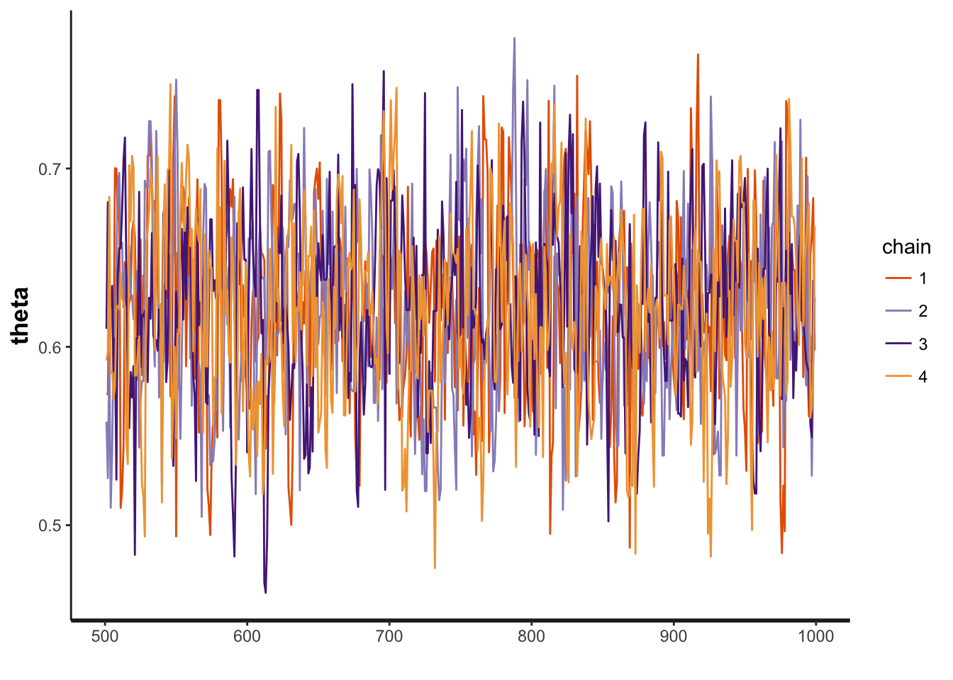

And if you want to get the sample from the model, you can use extract function.

theta_p <- extract(fit, "theta")
mean(theta_p$theta)

## [1] 0.6219672

Extract function will drop 50% of data in the warming up process.

Opimization

Stan also support optimization for research purpose, so that you can perform lasso or group lasso some penalized regression in stan. Just by adding log_increment to add in likelihood.

opt_stan <- optimizing(model_obj, data = dat)

## Initial log joint probability = -245.307
## Optimization terminated normally: 
##   Convergence detected: relative gradient magnitude is below tolerance

opt_stan$par

##      theta  ytheta[1]  ytheta[2]  ytheta[3]  ytheta[4] 
## 0.62682139 0.65670535 0.09329465 0.09329465 0.15670535

Stan in Lasso

Lasso in stan is also easy to code.

lasso_code <- "
data {
    int n;
    int p;
    vector[n] y;
    matrix[n, p] x;
    real<lower = 0> lambda;
}
parameters {
    vector[p] beta;
    real<lower = 0> sigma;
}
model{
    y ~ normal(x * beta, sigma);
    for (k in 1:p)
        target += -lambda * fabs(beta[k]);
}
"

p = 8
beta_true <- as.vector(c(3, 1.5, 0, 0, 2, 0, 0, 0))
sigma = matrix(0, p, p)
rho = 0.5
for(i in 1:p)
    for(j in 1:p)
        sigma[i, j] <- 0.5^(abs(i - j))
n = 20
x <- mvrnorm(n = n, mu = rep(0, p), Sigma = sigma)
y <- as.vector(x %*% beta_true + rnorm(n, 0, 2))

lambda = 3
stan_data <- list(n = n, p = p, y = y, lambda)

model_obj <- stan_model(model_code = lasso_code, model_name = "Lasso")

opt_stan <- optimizing(model_obj, data = stan_data)

## Initial log joint probability = -102.833
## Optimization terminated normally: 
##   Convergence detected: absolute parameter change was below tolerance

opt_stan$par

##       beta[1]       beta[2]       beta[3]       beta[4]       beta[5] 
##  1.263964e+00  1.633036e-01  4.758300e-10 -4.738927e-08  4.833109e-01 
##       beta[6]       beta[7]       beta[8]         sigma 
##  9.028171e-08  1.175658e-07  7.619844e-08  3.476164e+00

R stan example